
How to Calculate a Mold Tolerance Stack-Up
Table of Contents
A 20 mm pin-to-pin dimension on a connector housing came off the T1 tool at 20.045 mm against a print of 20.00 ±0.030 mm. The mold was not broken. Every individual component sat inside its own drawing limit, and the incoming inspection sheet for each part was clean. Five acceptable rings, added end to end, produced a part 0.015 mm outside specification. Correcting it meant re-cutting two cavity inserts, a new electrode set and three lost weeks before PPAP sampling could restart.
Tolerance stack-up is the arithmetic that catches that failure before steel is cut. It is also the tool that tells you whether a ±0.030 mm part print is a manufacturing instruction or a wish. This guide covers both calculation methods. It covers the five links that feed a mold chain. It also covers allocation of a part tolerance down to component limits. The final section lists the errors that let a stack-up pass review and still fail at T1.
The Snapshot
- Worst-case stack-up adds ring values. RSS adds them in quadrature, so ten equal ±0.010 mm rings give ±0.100 mm worst case and ±0.032 mm RSS.
- A five-ring mold chain of ±0.015, ±0.008, ±0.005, ±0.002 and ±0.020 mm resolves to ±0.050 mm worst case and ±0.027 mm RSS.
- Shrinkage compensation error is usually the largest ring: a ±0.10% resin rate uncertainty equals ±0.020 mm on a 20 mm dimension.
- CMM measurement uncertainty belongs outside the chain. Hold it under 10% of the tolerance, and guard-band the print if it grows past that.
- A ±0.020 mm shrinkage bias that RSS cannot see drops Cpk from 1.12 to 0.37 on the same ±0.030 mm print.
The 0.045 mm Gap That Stopped a T1 Build
The 0.045 mm in that first paragraph is not a typo. The gate dimension drifted 0.045 mm from nominal across an eight-cavity layout, and the print allowed only ±0.030 mm. Nobody had made a mistake that a single drawing check would catch. The mold base pocket sat 0.014 mm off nominal, inside its ±0.015 mm allowance. The insert-to-pocket fit added 0.007 mm of shift, inside ±0.008 mm. The core pin hole in the insert was 0.004 mm off true position, inside ±0.005 mm. The core pin itself was 0.002 mm off diameter and straightness, inside ±0.002 mm. Then the shrinkage factor of 0.40% turned out to be 0.45% on that cavity, worth 0.010 mm on a 20 mm dimension.
Every ring passed and the sum failed. That is the whole reason stack-up calculation exists. Drawings control components. Production ships assemblies, and an assembly carries the sum of every component error plus the process errors that no component drawing can hold. A 20 mm molded feature carries at least five contributors, and four of them are invisible on any single component print.
The cost mechanism is unforgiving because it arrives late. A stack-up error found at the drawing review costs one afternoon and a revised callout. The same error found at T1 costs far more. Electrode remakes run $800 to $2,500 per set. Insert re-cutting takes 40 to 80 machine hours. The PPAP calendar slides by 2 to 4 weeks. Found at PPAP, the cost is a full tool rework cycle. It also carries a customer confidence penalty that never appears on an invoice.
Buyers feel this most in automotive and connector work. A housing with 0.4 mm walls carries pin-to-pin dimensions at ±0.030 mm and true position at 0.05 mm. Those numbers are achievable. They are not achievable by accident, and they are not achievable by quoting each component at its own individual tolerance and hoping the sum behaves.
What a Mold Tolerance Chain Actually Contains
A mold tolerance chain is the ordered list of independent error sources between the machine table and the molded feature. Each ring carries a tolerance value, and every ring points at the same part dimension. The chain is written for one dimension at a time. The rings that matter for a pin spacing are not the rings that matter for a wall thickness or a sealing face.
Five ring families cover almost every injection mold chain. Steel machining tolerance covers every cutting operation on the plates and inserts, typically ±0.005 mm to ±0.020 mm depending on process class. Assembly and closure tolerance covers fits between inserts and pockets, leader pin to bushing clearance and side lock engagement, typically ±0.005 mm to ±0.015 mm. Shrinkage compensation error covers the gap between the factor in the CAD model and the rate the resin actually reaches. That gap typically runs ±0.10% to ±0.25% of the dimension. Parting face and core shift covers offset across the split line and core-to-cavity misalignment, typically 0.01 mm to 0.05 mm. Cavity count amplification covers cavity-to-cavity variation in a multi-cavity tool, typically ±0.01 mm to ±0.03 mm on a balanced layout.
Write the chain on one line before calculating anything. A usable chain entry has three fields: the ring name, the ± value in millimetres, and the physical reason the value is what it is. An entry that says "machining 0.01 mm" is not usable, because nobody can challenge it. An entry that says "cavity pocket position, jig-bored on a temperature-controlled machine, ±0.008 mm" can be challenged, verified and, if needed, improved. Stack-up disputes are almost always disputes about ring values, not about the arithmetic.
Keep the chain short and honest. A twelve-ring chain on a molded feature usually means the author was padding it, and padding does not change the answer much under RSS. It does inflate the worst-case number and make the print look unachievable. Four to seven rings is the working range for a single molded dimension. If your chain has more, most of those entries are measurement steps rather than manufacturing steps, and measurement steps belong in a different budget.
Worst-Case Stack-Up: The Additive Method
Worst-case stack-up is addition. For a chain of n rings, each with half-width T, the total is the sum of every ring at full limit in one direction. In formula form, T_wc = T1 + T2 + T3 plus every remaining ring to Tn. For the five-ring chain above, that is 0.015 + 0.008 + 0.005 + 0.002 + 0.020, which equals ±0.050 mm.
The method answers one question exactly. If every ring sits at its extreme limit simultaneously, does the part still conform? That is a guarantee, not an estimate, and it is the reason worst-case arithmetic dominates aerospace, medical and safety-critical molded parts. A bracket that holds a brake sensor connector must not fail because five suppliers all drifted the same way in the same week.
Worst-case is pessimistic by construction. It assigns zero probability to the middle of each ring. In reality a stable process spends most of its time near nominal, so the all-extremes case is rare but not impossible. The practical cost of that conservatism is real. On the five-ring chain, worst case says the chain needs ±0.050 mm of the print. If the print only allows ±0.030 mm, worst-case analysis declares the tool unbuildable. That forces tighter callouts on every ring and typically adds 15% to 40% to mold cost. The gain in shipped quality is often negligible.
Use worst-case when the part is safety-related or the volume is too low for a yield argument. Use it when one or more rings are biased rather than random. Use it whenever the customer specification demands it. Use it as a sanity floor on every chain even when you calculate RSS. The gap between the two numbers measures how much risk you are accepting.
RSS Stack-Up: The Statistical Method
Root sum square stack-up treats each ring as a random variable and combines standard deviations instead of limits. For independent rings, the variance of the sum equals the sum of the variances. The total is therefore the square root of the sum of squares. In formula form, T_rss = the square root of T1 squared plus T2 squared through Tn squared. For the same five rings, that is the square root of 0.000225 + 0.000064 + 0.000025 + 0.000004 + 0.000400, which equals ±0.0268 mm.
That is 54% of the worst-case value. The saving is not free, and the price is stated in four assumptions. Every ring must be independent of the others. Every ring must be roughly centred on nominal, with no systematic bias. Every ring must be approximately normally distributed, which requires a capable, stable process. Every ring's tolerance value must correspond to a known number of standard deviations, conventionally three.
When those assumptions hold, RSS is the more accurate model and the more useful one. It explains why a real shop can build a ±0.030 mm tool from components held at ±0.050 mm of total chain error. It also explains why that shop occasionally fails. RSS describes a distribution. Roughly 99.7% of builds will land inside three standard deviations if the assumptions survive.
Verify the assumption before you trust the number. Measure thirty parts per cavity at steady state and compute the standard deviation of each ring you can measure. If the measured combined three sigma exceeds the predicted value by more than 30%, one ring is biased or one process is out of control. Predicted three sigma on the five-ring chain is 0.0268 mm, so a measured value above 0.035 mm is a finding, not noise.
Five-Ring Example: Worst Case vs RSS
Take a glass-filled PA66 connector housing with an 8-cavity tool and a critical pin-to-pin dimension of 20.00 ±0.030 mm. The mold is built plate first, pockets jig-bored on a temperature-controlled machine, and inserts finished on a wire EDM. The chain carries five rings, listed below with the cumulative result after each one.
| Ring | Error source | ± value | Worst case | RSS |
|---|---|---|---|---|
| 1 | Mold base pocket position, jig-bored | ±0.015 mm | ±0.015 mm | ±0.0150 mm |
| 2 | Insert to pocket fit and side lock engagement | ±0.008 mm | ±0.023 mm | ±0.0170 mm |
| 3 | Cavity insert feature machining, core pin hole true position | ±0.005 mm | ±0.028 mm | ±0.0177 mm |
| 4 | Core pin diameter and straightness | ±0.002 mm | ±0.030 mm | ±0.0178 mm |
| 5 | Shrinkage compensation error at ±0.10% on 20 mm | ±0.020 mm | ±0.050 mm | ±0.0268 mm |
← swipe to scroll →
Table note: values are typical industry figures for a precision connector mold built on a plate-first process, not DieStrike capability limits. The worst-case column adds ring values, the RSS column shows the root sum square of all rings up to that row.
Read the RSS column and the design argument appears. Rings 1 through 4 build a combined RSS of ±0.0178 mm, and ring 5 alone more than doubles it to ±0.0268 mm. Tightening the mold base pocket from ±0.015 mm to ±0.008 mm moves the worst-case number by 0.007 mm and the RSS number by 0.0035 mm. Tightening the shrinkage estimate from ±0.10% to ±0.05% moves RSS by 0.0068 mm. On this chain, the arithmetic points at the resin, not the grinder.
Convert the number into a capability index. If each ring tolerance equals three standard deviations, the RSS value is the three sigma width of the sum. Split the two limits, so Cpk equals the distance from nominal to the nearest limit divided by three sigma. Against a ±0.030 mm print, Cpk is 0.030 divided by 0.0268, which is 1.12. Against a relaxed ±0.050 mm print, the same chain yields Cpk 1.87. That is the calculation that decides whether a part print ships or gets renegotiated.
Two hybrid rules appear in shop practice when one ring dominates. The first takes the largest ring at full value and adds the RSS of the rest, which gives 0.020 plus 0.0178, or ±0.0378 mm. The second multiplies the full RSS by 1.5, which gives ±0.0402 mm and approximates a four to four-and-a-half sigma bound. Both sit above the RSS answer and below the worst-case answer, and both are reasonable when the dominant ring is suspected of bias.
The Five Links That Feed a Mold Chain
Link one is steel machining tolerance. The value depends on process class, not on effort. CNC milling on a plate reaches ±0.015 mm to ±0.020 mm. Jig boring on a temperature-controlled machine reaches ±0.008 mm to ±0.010 mm. Surface grinding and wire EDM on a machine held within ±1 °C reach ±0.003 mm to ±0.005 mm. Precision molds run at ±0.005 mm on critical tool dimensions, with individual component geometry at ±0.002 mm where the process supports it.
Link two is assembly and closure tolerance. Inserts need clearance to enter a pocket, and that clearance becomes position error. A typical slip fit adds 0.005 mm to 0.010 mm, and a bolted insert with dowel location removes most of it. Leader pin to bushing clearance runs 0.010 mm to 0.025 mm diametral on a standard mold. Each of the four pins contributes a fraction of that as plate shift during closure. Side locks with a 3° to 7° engagement face typically add 0.005 mm to 0.015 mm at the cavity. Their absence on a high-cavity tool shows up as a closure ring worth 0.02 mm or more.
Link three is shrinkage compensation error. This ring carries the gap between the shrinkage factor in the CAD model and the rate the resin reaches. Uncertainty of ±0.10% on a 20 mm dimension equals ±0.020 mm. The same ±0.10% on a 100 mm dimension equals ±0.100 mm, which is why long molded dimensions are almost always shrinkage-limited. No amount of jig boring fixes that ring.
Link four is parting face offset and core shift. A well-built precision mold holds parting face mismatch at 0.02 mm to 0.03 mm and core-to-cavity coaxiality at 0.01 mm to 0.03 mm. Both feed directly into any dimension that crosses the split line or depends on wall thickness around a core pin. Shut-off geometry amplifies the effect, because a 0.01 mm height mismatch on a 5° shut-off face moves the resulting edge laterally by 0.11 mm.
Link five is cavity count amplification. In a multi-cavity tool, cavity-to-cavity dimensional spread is a separate ring measured as max minus min across cavities. A balanced 8-cavity layout typically spreads 0.005 mm to 0.030 mm. The stack-up uses the worst cavity, so the ring value is the full spread and not the average. That ring applies once, not once per cavity.
Shrinkage Compensation Error: The Largest Ring
Shrinkage compensation error earns its own section because it is both the biggest ring and the one treated most casually. A mold designer picks a factor, often from a resin supplier data sheet, and writes it into the model. The data sheet gives a range, not a value. Polypropylene spans 1.0% to 2.5%. Glass-filled PA66 spans 0.2% to 0.6%. Polycarbonate sits at 0.5% to 0.7%, and acetal at 1.8% to 2.5%.
Even inside one grade, the rate moves with wall thickness, gate location, melt temperature, packing pressure and fiber orientation. A ±0.10% band is a reasonable estimate for a well-characterised grade in a simple geometry. A complex housing with 0.4 mm to 2.5 mm walls and side-gated fiber-filled resin can swing ±0.25%. On a 60 mm dimension that is ±0.150 mm on its own.
Match the ring value to the geometry, not to the data sheet. Two rules keep this ring honest. First, apply the uncertainty in millimetres at the actual dimension under study, because a percentage is meaningless until it is multiplied. Second, split the factor by flow direction for fiber-filled resins. A 30% glass-filled grade can run 0.25% along flow and 0.75% across flow. One averaged factor hides a 0.5% error.
Shrinkage error is usually a bias, not a scatter. This is the single most important fact about the ring. If the factor is 0.40% when the resin runs at 0.45%, every cavity shifts the same way. A biased ring moves the mean of the sum, and RSS arithmetic assumes a centred mean. That is why the statistical model can look comfortable on paper and still ship parts outside limit.
The fix costs one trial and pays for itself. Run a T0 short shot or a full T1 sampling with the production resin, gate position and cooling layout. Measure at least 30 parts per cavity and back-calculate the real rate per dimension. That typically pulls the uncertainty from ±0.10% to ±0.05% and removes the bias term. Our guide on shrinkage compensation rules covers the per-dimension method and the correction order.
How Cavity Count and Core Shift Enter the Chain
Cavity count changes the risk profile more than it changes the arithmetic. The per-dimension spread across an 8-cavity tool enters the chain once, as a single ring of 0.005 mm to 0.030 mm. A common and expensive mistake is to multiply that ring by the square root of the cavity count. That turns a ±0.020 mm ring into ±0.057 mm and declares a perfectly buildable tool impossible.
The real cavity-count effect is in the probability that at least one cavity drifts beyond a ring limit. If each cavity carries an independent 0.5% chance of drifting, the chance that at least one of eight does is 3.9%. At 32 cavities the same per-cavity risk becomes 14.8%, and at 64 cavities it reaches 27.4%. The arithmetic of the chain is unchanged. The exposure is not.
Core shift behaves like a wall thickness ring. Uneven melt pressure around a core pin bends it, so the molded wall on one side thickens while the other thins by the same amount. Flow-induced core shift typically runs 0.02 mm to 0.10 mm on an unsupported slender core at high fill rates. The mold-side contribution, meaning core pin coaxiality, pin straightness and support length, is held at 0.01 mm to 0.03 mm on a precision tool. Insist on both numbers separately, because the fix differs. Coaxiality is a machining problem, and flow-induced shift is a gate and fill-balance problem.
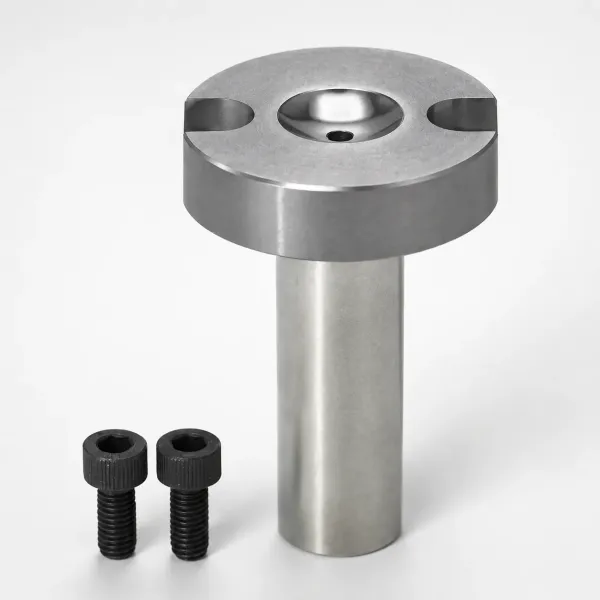
Thermal asymmetry sets a floor on the spread. Coolant circuits that differ by 10 °C between cavities typically shift the local shrinkage rate by 0.03% to 0.08%. That equals 0.006 mm to 0.016 mm on a 20 mm dimension. That is the same order as the best cavity-to-cavity machining spread. A tool with an imbalanced cooling layout cannot be rescued by tighter steel work. Balance the circuits to within 3 °C before spending money on jig boring.
Record the spread as a specification, not a hope. Quote the tool with a stated cavity-to-cavity spread limit, for example 0.020 mm max minus min across eight cavities at steady state. That single number gives the stack-up a real ring value. It also gives the moldmaker a measurable target at T1. It gives you a contractual basis to reject a tool that ships with one drifting cavity.
Tolerance Allocation: From Budget to Component Limits
Allocation runs the calculation backwards. You start with the print tolerance and the capability you need, convert both into a three sigma budget, then divide that budget among the rings. If the print is ±0.030 mm and the customer requires Cpk 1.33, the budget is 0.030 divided by 1.33. That equals ±0.0226 mm of chain three sigma. If the customer requires Cpk 1.67, the same print allows only ±0.0180 mm.
The equal-allocation rule gives a starting split for a new design. For n independent rings, each gets the budget divided by the square root of n under RSS. A five-ring budget of ±0.0226 mm therefore assigns ±0.0101 mm to each ring. That number is achievable for four of the five rings. It is impossible for the shrinkage ring. Allocation is therefore a negotiation with physics rather than a division problem.
| Option | Rings after change | Chain 3 sigma | Cpk vs ±0.030 mm | Cost and lead time |
|---|---|---|---|---|
| Baseline, no change | 0.015, 0.008, 0.005, 0.002, 0.020 | ±0.0268 mm | 1.12 | Reference |
| A. Jig-bore pockets to ±0.008 mm | 0.008, 0.008, 0.005, 0.002, 0.020 | ±0.0236 mm | 1.27 | +8% to 12% mold price |
| B. Machine core pin holes after assembly | 0.005, 0.002, 0.020 | ±0.0207 mm | 1.45 | +3% to 5% mold price |
| C. Shrinkage DOE at T0, band ±0.05% | 0.015, 0.008, 0.005, 0.002, 0.010 | ±0.0204 mm | 1.47 | 2 weeks trial |
| D. Option B plus option C | 0.005, 0.002, 0.010 | ±0.0114 mm | 2.64 | +3% to 5% and 2 weeks |
← swipe to scroll →
Table note: chain three sigma values are the root sum square of the rings listed, in millimetres. Cpk assumes a centred mean and equals 0.030 mm divided by the chain three sigma. Cost figures are typical industry ranges, not DieStrike quotations.
Read the table as a decision ladder. Option A buys 0.0032 mm of statistical margin for a 8% to 12% price increase and still misses Cpk 1.33. Option B removes two rings from the chain by machining the core pin holes in place after assembly. That cuts the chain by 23% for a 3% to 5% cost increase. Option C attacks the biased ring and lands at Cpk 1.47. Option D combines both and reaches Cpk 2.64, at which point the print could be tightened rather than relaxed.
Allocation rules that survive contact with a shop floor follow three principles. Give the tight budget to the process that controls it cheaply, which is usually wire EDM or grinding on an insert. Give the loose budget to the ring that is expensive to control, which is usually assembly clearance. Never allocate a budget the resin cannot meet. A shrinkage ring quoted at ±0.005 mm on a 60 mm dimension is a promise nobody can keep.
Ask your moldmaker for the chain when you issue a tight print. A DFM review that returns a ring-by-ring budget with named processes is worth more than any statement that a tolerance is achievable. Our mold design and DFM service returns that budget inside 24 hours, before any electrode is cut.
Five Stack-Up Errors That Pass Inspection
Error one is using RSS to hide a biased ring. Keep the five-ring chain and add a 0.020 mm systematic shift to the shrinkage ring, which is what a wrong factor produces. The RSS value stays at ±0.0268 mm because the calculation cannot see a mean offset. Against a ±0.030 mm print, Cpk falls from 1.12 to 0.37. The failure rate moves from a rare tail event to a normal production outcome. Any ring that can be biased must be reported at full value, not in quadrature.
Error two is mixing CMM measurement uncertainty into the budget. A CMM stated at MPE 1.5 + L/350 µm resolves about 1.56 µm at a 20 mm length. Expanded uncertainty with fixturing and thermal effects typically lands at 2 µm to 4 µm. That uncertainty is not a manufacturing ring. Adding it to the chain inflates the budget and drives unnecessary machining. Ignoring it entirely is the opposite error. The working rule is a test uncertainty ratio, keeping measurement uncertainty under 10% of the tolerance width and guard-banding the print when it exceeds that. A ±0.030 mm print tolerates a 0.006 mm uncertainty. A ±0.005 mm print demands 0.001 mm, which no CMM delivers, so the check moves to a comparator stand, air gauge or gauge blocks. Our guide on reading a CMM report covers how to find the uncertainty statement on a measurement sheet.
Error three is adding correlated rings in quadrature. RSS requires independence. Four inserts machined in one setup on one machine, at one temperature, share a common error. If that common error is 0.005 mm, treating the four as independent rings understates the sum. The correction is to declare the shared component as one ring at full value and only the independent residuals as separate rings.
Error four is mixing unilateral and bilateral callouts. A ring written as +0.050 mm and 0 mm has a half width of 0.025 mm only if the process sits mid-zone. A unilateral callout rarely sits mid-zone. Worst-case addition uses the full width in the worst direction, while RSS needs a centred half width. Mixing the two conventions inside one chain produces a number that is neither a guarantee nor a distribution, and it usually understates the real risk.
Error five is applying RSS to a process that is not capable. Quadrature assumes each ring behaves like a centred normal variable with the tolerance equal to three sigma. That requires Cpk of at least 1.33 on every ring. A ring running at Cpk 0.80 has a heavy tail, and the RSS answer will be optimistic by 30% or more. Check ring capability before you use the statistical method, and fall back to worst case on any ring you cannot measure.
Stack-Up Limits at ±0.005 mm and ±0.002 mm
Precision mold work draws a line that stack-up arithmetic makes visible. A mold can hold ±0.005 mm on critical tool dimensions and ±0.002 mm on individual component geometry. Cavity inserts are heat treated to HRC 62 for wear resistance. Those numbers define the mold-side rings in any chain, and they set a hard floor on what the tool alone contributes.
Put the two mold-side rings into the arithmetic. A ±0.005 mm machining ring plus a ±0.002 mm component ring yields an RSS of ±0.0054 mm. That is the mold-only floor for a dimension that depends on machining and assembly accuracy alone. Add a shrinkage ring of ±0.010 mm from a trial-backed rate band and the chain reaches ±0.0114 mm. Add ±0.020 mm instead and it reaches ±0.0207 mm. So a molded dimension quoted at ±0.015 mm is a realistic target. A molded dimension at ±0.005 mm is a demand on the resin and the process window, not on the mold shop.
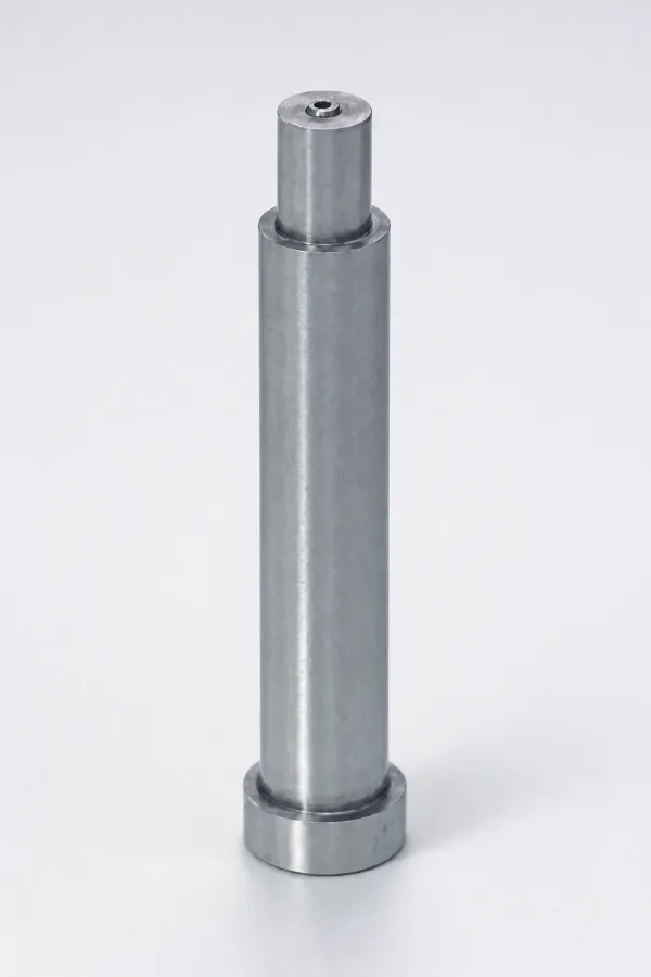
Heat treatment is a ring that buyers forget. Hardening and tempering a cavity insert at 48 to 52 HRC typically distorts 0.005 mm to 0.015 mm per 100 mm of length. Vacuum hardening adds another 0.002 mm to 0.005 mm of size change. Any dimension that must be final after hardening has to be ground or wire-cut after heat treatment. That correction step belongs in the chain as a named operation, not as an assumption. Our guide on holding ±0.002 mm tolerances covers the machine class and thermal control behind those numbers.
Validate the stack-up at end of life, not only at T1. Shut-off faces on a tool running 500,000 cycles wear 0.005 mm to 0.020 mm, and that wear enters the parting face ring over time. A chain that closes at Cpk 1.45 on day one can drop below 1.33 by mid-life if wear consumes 0.010 mm of the parting ring. Budget the wear, schedule the shut-off check, and treat the stack-up as a life-cycle calculation.
FAQ: Mold Tolerance Stack-Up
Q1. What is the difference between worst-case and RSS tolerance stack-up?
Worst case adds every ring at its full limit, which on a five-ring chain of ±0.015, ±0.008, ±0.005, ±0.002 and ±0.020 mm gives ±0.050 mm. RSS adds the squares and takes the root, which gives ±0.0268 mm, or 54% of the worst-case value. Worst case is a guarantee. RSS is a probability statement that requires independent, centred and capable rings.
Q2. Is RSS or worst-case required for automotive mold tooling?
Most automotive and connector customers accept a statistical stack-up when every ring holds Cpk 1.33 or better. The analysis must also be documented in the PPAP package. Safety-critical features and any ring with a known bias are usually required to pass worst case. On the five-ring example, the ±0.030 mm print passes at Cpk 1.12 under RSS. It needs either a tighter ring or a Cpk 1.33-capable process before it is defence-able.
Q3. How many rings should a mold tolerance chain contain?
Four to seven rings for a single molded dimension. Fewer than four usually means a real error source was omitted, most often shrinkage compensation error. More than seven usually means measurement and handling steps were mixed into a manufacturing chain. That inflates the worst-case total without changing the statistical result much.
Q4. Should CMM measurement uncertainty be added to the tolerance stack-up?
No. Measurement uncertainty is a verification budget, not a manufacturing ring. Keep it under 10% of the tolerance width and guard-band the part limits when it grows beyond that. A CMM resolves about 1.6 µm at a 20 mm length. That is fine for a ±0.030 mm print and not fine for a ±0.005 mm print.
Q5. Why did my tool pass every component inspection and still miss the part print?
Because component inspection checks rings one by one and the part print constrains the sum. A chain of ±0.015, ±0.008, ±0.005, ±0.002 and ±0.020 mm sums to ±0.050 mm worst case even when every component is inside its own limit. When the shrinkage factor is wrong by 0.05%, the ring that failed is the one nobody measured at T0. That ring carries 40% of the total chain.
The Bottom Line
A mold tolerance stack-up is a contract review, not a formality. Calculate worst case for the guarantee and RSS for the strategy, then attack the shrinkage ring before the grinder. A ±0.030 mm print on a ±0.027 mm chain is a 1.12 Cpk part, and no inspection plan fixes that. Send us your print and we will return the ring budget.
Have a tight print that keeps failing at T1? Send it to our engineering team and we will run the chain ring by ring before any steel is cut.
KEEP READING
Related Reading
How to Hold ±0.002mm: Precision Mold Tolerances
What it actually takes to hold ±0.002 mm on mold components: machine class, temperature control, steel stability and CMM verification order.
Read articleArticleHow to Read a CMM Report: Dimensional Data for Mold Buyers
Nominal vs actual vs deviation, true position as a diameter, Cp and Cpk at 1.33 and 1.67, and the 23 ±1 °C rules behind every CMM sheet.
Read articleArticle5 Shrinkage Compensation Rules for Mold Design
Five rules for shrinkage factors, from rate ranges by resin family to gate and fiber orientation effects on final molded dimensions.
Read articleServiceMold Design and DFM
24-hour DFM feedback on your part print: datum scheme, tolerance feasibility, shrinkage compensation and steel selection before cutting starts.
Read articleNEXT STEP
Ready to Start Your Mold?
Send us your element dimensions or part numbers — our team responds within 24 hours with pricing and lead time.

Written by
Ray ChanMold Buyer's Guide Author · Precision Mold Manufacturing Specialist. Ray helps global importers, distributors and OEMs source factory-direct molds and mold parts.